


The Galileo Energetic Particles Detector
Galileo EPD Handbook
Chapter 1. Instrument Summary
Charged Particle Response of Magnetic Deflection System for Galileo Jupiter Orbiter (draft) (continued)
Results of the Simulation
The mapping in Figure 8 shows that the angular distributions have a correlation between an electron detector and the apertures. The particles emanating from those points (z=0.0) have a symmetric distribution due to the symmetry of the magnetic field with respect to the middle plane. Because of this property, scanning both polar and azimuthal angles at a sample point away from the middle plane should yield the same number of detected particles as the number obtained from the sample point from the opposite side of the middle plane. The angular distributions for these two opposite points should also be the same. The demonstration of this symmetry is given in Figures 9a and b in terms of angular distributions of both 50 keV electrons and 25 keV protons with respect to the middle plane. This can also be shown for other energies, and, in fact, this property is used to reduce a substantial amount of computer time.
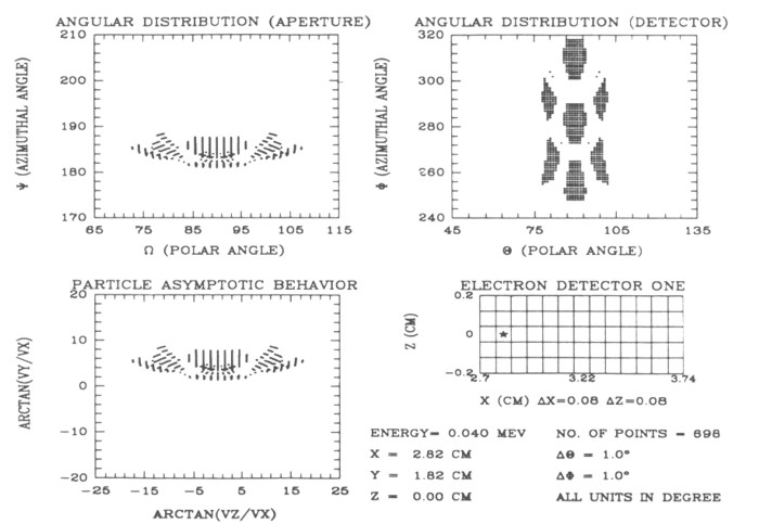 |
Figure 8. The mapping of angular distributions at detector E and apertures. |
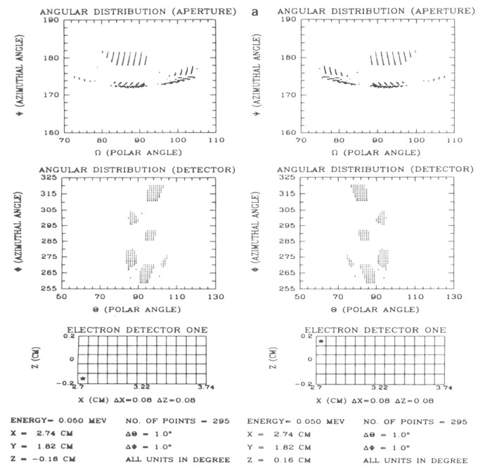 |
Figure 9a. Angular distributions of 50 keV electrons for two symmetric sample points with respect to the middle plane. |
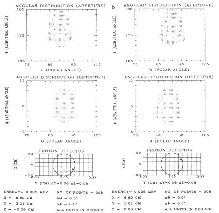 |
Figure 9b. Angular distributions of 25 keV protons for two symmetric sample points with respect to the middle plane. |
This simulation shows that high energy electrons are separated from low energy electrons and protons are separated from electrons. For electron detector E, the low limit for electrons to be detectable occurs at approximately 20 keV. High energy electrons such as 600, 800, and 1000 keV are still detectable but in a very small number. For electron detector F, the low limit is at 100 keV with only eight electrons detected. Protons deflect very little and 5 keV is the approximate low energy limit. The number of electrons at each sample point on detectors E and F varies significantly as the sample point moves away from the apertures, with maximum and minimum values being observed. The proton detector has a similar variation in detected particle numbers. The numerical values are provided elsewhere [10].
Emanating from a sample point on the detector, higher energy electrons are deflected less than are lower energy electrons by the magnetic field. As a consequence, they are expected to have smaller azimuthal angles than lower energy electrons at the apertures. (The polar and azimuthal angles θ and φ are defined as the conventional spherical coordinate system.) As shown in Figure 9c, this simulation indeed demonstrates this feature; the azimuthal angles of 50 keV electrons range from 191° to 197° and those of 80 keV electrons range from 176° to 191°. For 100 keV electrons the range is from 171° to 189°.
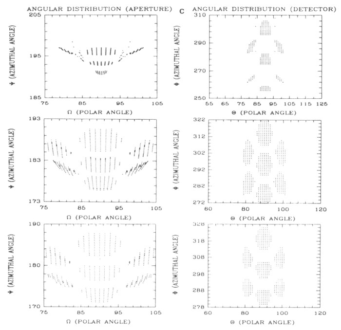 |
Figure 9c. Comparison of the angular distributions for 50 (top), 80 (center), and 100 keV (bottom) electrons emanating from the center of detector E with x=3.22 cm and y=1.82 cm. |
With the acquisition of the total number of particles counted by a detector, we can compute the geometric factors by applying equation (7). In the polar coordinates used the polar axis lies in the detector plane. The angle θ for open trajectories in all cases provided is close to 90°, which makes the factors sin(θi + ½Δθi) all approximately equal to 0.995 ±0.003. The numbers of detected particles at those uncalculated sample points are obtained by third-order spline interpolation. Therefore, for these points, the factor is not available. Since this factor has no significant effect on the final results, we decided to use the average value; the equation for the geometric factors now becomes:
![]()
where N is the total number of particles counted by a detector for a particular energy and
<sin(θi + ½Δθ)> is the average value. The geometric factor is customarily expressed as cm2 sr.
In our calculation Δθ and Δφ take the value of one degree interval. The final results of the geometric factors are listed in Table 1 and plotted in Figure 10. We also use the third-order spline interpolation method to infer the geometric factors for other energies. The threshold values of the geometric factors for the proton detector and for electron detectors E and F are 5, 20, and 100 keV, respectively. The maximum values (interpolated) for electron detectors E and F occur at 70 and 500 keV, respectively. As expected, the geometric factor for the proton detector increases monotonically since the proton detector is placed directly in line with the open apertures and high energy protons can almost go through the detector without much deflection. For a desired energy, the calculation can be performed to obtain very accurate results.
Table 1. The geometric factors of the Galileo LEMMS detectors.
| Type of Detector |
Energy (keV) |
Number of Particles |
Geometric
Factors [sr cm2] |
| Electron Detector E | 20 | 1175 | 0.002279 |
| 30 | 7027 | 0.013631 | |
| 40 | 13370 | 0.025935 | |
| 50 | 16125 | 0.031279 | |
| 80 | 17598 | 0.034137 | |
| 100 | 16919 | 0.032820 | |
| 200 | 8645 | 0.016770 | |
| 400 | 2397 | 0.004650 | |
| 600 | 1146 | 0.002223 | |
| 800 | 656 | 0.001272 | |
| 1000 | 402 | 0.000780 | |
| Electron Detector F | 100 | 8 | 0.000016 |
| 200 | 2015 | 0.003909 | |
| 400 | 9112 | 0.017675 | |
| 600 | 9417 | 0.018267 | |
| 800 | 7919 | 0.015381 | |
| 1000 | 7370 | 0.014296 | |
| 3000a | 2662 | 0.005164 | |
|
Proton Detector (12.57 mm2 used)b |
5 | 385 | 0.000747 |
| 15 | 1253 | 0.002431 | |
| 20 | 1341 | 0.002601 | |
| 25 | 1382 | 0.002681 | |
| 50 | 1457 | 0.002826 | |
| 75 | 1559 | 0.003024 | |
| 1000 | 1574 | 0.003053 |
a This energy has not
been used for interpolation.
b An area of 24.63 mm2 will
also be used for the proton flight detector.
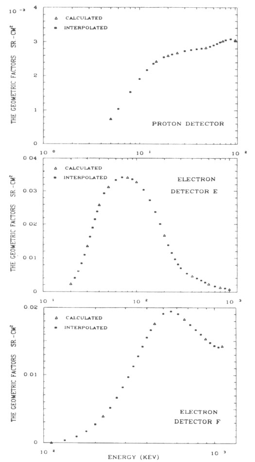 |
Figure 10. Geometric factors of detectors of the Galileo LEMMS sensor. |
Next: Conclusions
Return to Galileo EPD Handbook Table of Contents Page.
Return to main
Galileo Table of Contents Page.
Return to Fundamental
Technologies Home Page.
Updated 8/23/19, Cameron Crane
QUICK FACTS
Mission Duration: Galileo was planned to have a mission duration of around 8 years, but was kept in operation for 13 years, 11 months, and 3 days, until it was destroyed in a controlled impact with Jupiter on September 21, 2003.
Destination: Galileo's destination was Jupiter and its moons, which it orbitted for 7 years, 9 months, and 13 days.