Investigation of the Magnetosphere of Ganymede with Galileo's Energetic Particle Detector

Ph.D. dissertation by Shawn M. Stone, University of Kansas, 1999.

Copyright 1999 by Shawn M. Stone.  Used with permission.

1.2.1 Radial Diffusion Coefficients

The absorption signatures due to satellites have been used to calculate radial diffusion coefficients in the magnetospheres of Jupiter and Saturn [Mogro-Campero and Fillius, 1976; Thomsen et al., 1977; Van Allen et al., 1980; Simpson et al., 1980; Carbary et al., 1983]. The signatures are labeled either as a macrosignature or microsignature. The different distinctions between these two types of signatures are important. Macrosignatures are the result of repeated encounters of trapped radiation with the satellite. The effects are averaged over a long time scale (quasi-stationary state) [Van Allen et al., 1980]. Macrosignatures generally have a spatial extent of many satellite radii [Bell, 1989]. Microsignatures are absorption features that reflect the most recent interaction with the satellite and then drift in longitude via corotation, curvature, and gradient drifts. The absorption appears as a shadow that drifts in longitude at the drift rate of the missing particles. The shadow is eventually filled in by particles diffusing radially between L shells in response to magnetic or electric fields or progressively washed out by pitch angle or energy dispersion in the drift rate [Van Allen et al., 1980]. As a result of these processes, the shadow becomes shallower as it drifts in longitude until it is filled in completely. Knowing, then, the position of the spacecraft in longitude from the satellite, the coefficient of radial diffusion can be calculated.

Particles are transported radially between L shells by the violation of the third adiabatic invariant in a process called radial diffusion [Shulz and Lanzerotti, 1974; Walt, 1994]. Radial diffusion can be modeled by the one dimensional diffusion equation

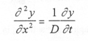
where y(x,t) is the one dimensional normalized count rate, x is the radial distance, t is the time, and D is the coefficient of radial transport [Van Allen et al., 1980].

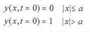
To solve Equation [1.9] an initial (t=0) profile of the normalized signature is needed. The assumption made is shown in Figure 1.6. For a satellite of radius a where the gyroradius of the particle is ρ~>a, the initial conditions are approximated by

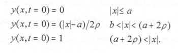
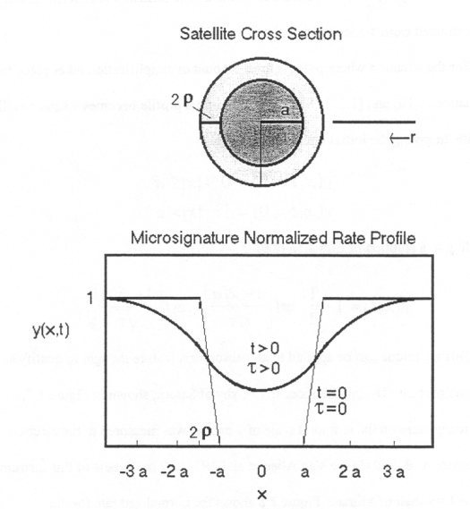
Figure 1.6 (A) Satellite cross-section in the radial direction. Particles are completely absorbed if their trajectories fall within the radius of the satellite x<a. For particles within two gyroradii of the surface of the satellite 2 ρ, there is a finite probability that they will be absorbed. (B) The normalized rate profile for a microsignature caused by the satellite. τ=0 represents the initial gyrophase averaged profile for the signature. As time increases τ>0 the microsignature drifts in longitude and fills in from diffusion, becoming broader and shallower.

If we define the dimensionless quantity

where t is the longitudinal drift time from the satellite to the spacecraft, and D and a are as before, the solution to Equation [1.9] is then of the form

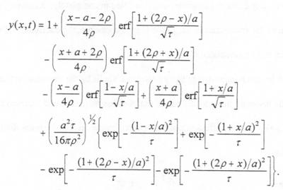
Equation [1.12] describes empirically the filling in of the signature as it drifts in longitude from the satellite. For increasing time, from t=0 to t>0, the signature fills in and becomes broader and shallower (as shown in Figure 1.6) until it disappears. It is then possible to least squares fit a microsignature to Equation [1.12] by inputting ρ and a and varying τ until a minimum is reached. The diffusion coefficient D can then be extracted from τ once t is calculated.

For the situation where ρ<<a, a great amount of simplification takes place for Equations [1.10] and [1.12]. Since r-0, the initial profile becomes a square well of width 2a giving the initial conditions

leading to a solution of Equation [1.9]:

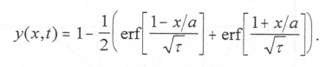(1.14)

This technique can be applied to any absorption feature thought to qualify as a microsignature. During the Pioneer 11 flyby of Saturn, shown in Figure 1.7, a microsignature on the temporal scale of 1 minute was measured in the electron detectors A, B, and C (see Van Allen et al.[ 1974] for the details of this instrument) at the L=3 shell of Mimas. Figure 1.8 shows the normalized rate for the microsignature of Mimas vs. Earth received time for the electron A, B, and C detectors. The solid line represents the best fit for the Mimas microsignature, given the parameters of the moon (a=180 km) and the gyroradius of ρ=10 km for 1.7 MeV electrons which gives τ=12. To extract the radial diffusion coefficient, the drift velocity of 1.7 MeV electrons was used at the orbit of Mimas, giving a drift time of t=6.44 hrs. This yields a diffusion coefficient of D=3.9 x 10^-10 R_s² s^-1, which is somewhat of an upper bound since dispersion has not been included as a possible fill-in mechanism [Van Allen et al., 1980].

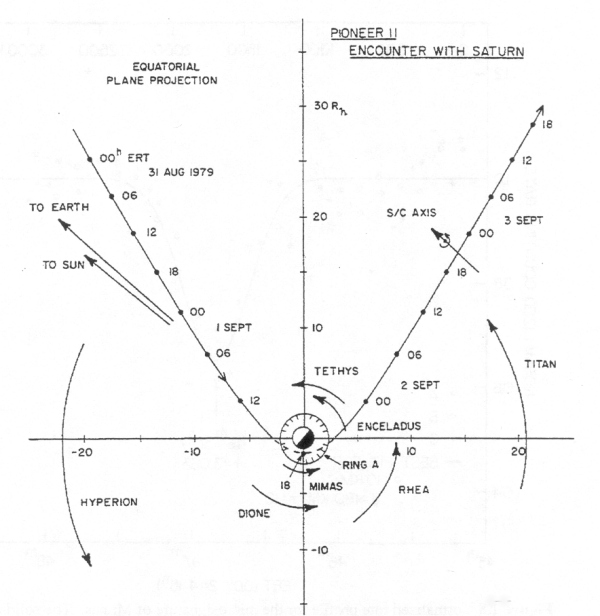Figure 1.7 Equatorial plane projection for the Pioneer 11 encounter at Saturn. Shown are the L shells of the satellites as Pioneer 11 crossed them.

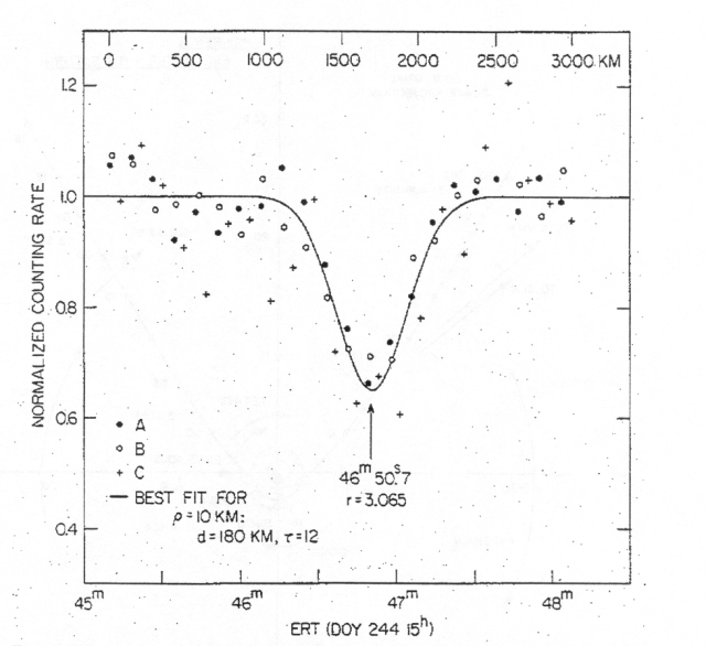Figure 1.8 Normalized rate profile for the microsignature of Mimas. The solid curve is the best fit result of the simple 1D diffusion equation of satellite sweepup and refilling process for the case of total initial absorption and a particle gyroradius of ρ=10 km.

Another good example is given by Voyager, which witnessed several microsignatures in the Saturnian magnetosphere. The Voyager spacecraft had a much better particle instrument called the low-energy charged particle instrument (LECP). It was capable of measuring energetic electrons (14 keV<=E<10 MeV) and ions (30 keV<=E <150 MeV) and it unambiguously separates electrons from ions in most cases [Krimigis et al., 1977]. For the satellite Dione, during the Voyager 1 flyby (Figure 1.9) a strong microsignature was seen in the two lowest energy channels only (26-37 keV and 37-70 keV) [Carbary et al., 1983]. At the orbit of Dione, the gyroradii for these energies are ρ<~10 km, so to calculate the diffusion coefficient Equation [1.14] can be utilized. Figure 1.10 shows the normalized count rate for 3 electron passbands of the LECP detector, 26-37, 37-70, and 70-130 keV. The angular drift speed relative to Dione is calculated to be 1 x 10^-4rad/s which gives t=4000 s for the drift time from the satellite to Voyager 1 and the radius of Dione is a=560 km. Figure 1.10 shows the fit to Equation [1.6] giving τ=10 for 26-27 keV electrons and τ=50 for 37-70 keV electrons. Using the drift time of t=4000 s for each gives D=5 x 10^-8 R_s² s^-1 and D=3 x 10^-7 R_s² s^-1 respectively [Carbary et al.,1983].

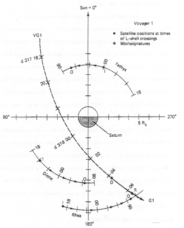Figure 1.9 Equatorial plane projection of the trajectory of Voyager 1 through the magnetosphere of Saturn. Heavy dots on the orbits of the satellites indicate its position when Voyager 1 crossed its L shell inbound (I) and outbound (O). Asterisks that appear on the trajectory of the spacecraft indicate times when satellite-associated microsignatures occurred.

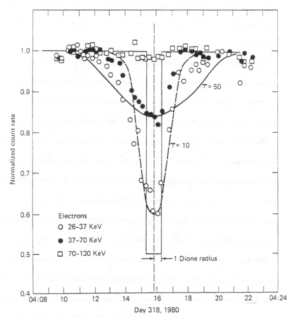Figure 1.10 Normalized electron rate profile for three energy passbands of the LECP instrument at Dione for Voyager 1. The best fit for 26-37 keV electrons gives τ=10, and for 37-70 keV electrons τ=50.

Next: 1.2.2 Magnetic Field Geometries

Return to dissertation table of contents page.

Return to main Galileo Table of Contents Page.
Return to Fundamental Technologies Home Page.

QUICK FACTS

RELATED LINKS