Investigation of the Magnetosphere of Ganymede with Galileo's Energetic Particle Detector

Ph.D. dissertation by Shawn M. Stone, University of Kansas, 1999.

Copyright 1999 by Shawn M. Stone.  Used with permission.

2.5 Electric Fields

The sources of electric fields in the magnetosphere are due to two mechanisms: changing magnetic fields and a non-uniformity in the spatial and velocity distribution between electrons and ions. Electric fields affect charged particle distributions by accelerating them. The direction of acceleration depends, of course, on the orientation of the particle’s motion relative to the electric field vector. In this section two types of electric fields will be discussed that are integral to this work. The first is a field oriented parallel to the magnetic field direction which occurs from the difference between the ion and electron pitch angle distributions. The second is a field oriented perpendicular to the magnetic field induced from the rotation of a planet’s magnetic field, called corotational electric field.

2.5.1 Parallel Electric Field

When a plasma is immersed in a homogenous magnetic field and a parallel electric field is applied along it, ions and electrons are accelerated until E_|| cancels out as shown in Figure 2.11a. However, a magnetic field with a mirror configuration such as the Earth’s dipole field (Figure 2.11b) with a potential difference between the equator and the ends of each field line no longer produces such a simple unidirectional shift when E_|| is applied [Stern, 1981]. Persson [1963, 1966] has shown that even under these circumstances an equilibrium can still exist in which the particles move with a non-vanishing E_||. Since the trajectories of ions and electrons react to E_|| in different ways, the entire distribution must be integrated over all velocity space, and Persson found charge neutrality was maintained at every point despite the presence of E_||.

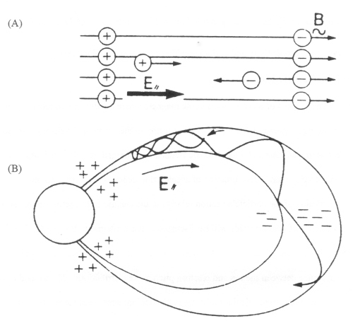Figure 2.11 A schematic diagram showing how electrons and ions respond to electric fields. (A) Homogeneous magnetic fields tend to cancel E||. (B) Inhomogeneous magnetic fields such as the Earth's dipole field can maintain an E|| [Stern, 1981].

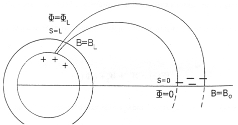
Let's consider what effect a parallel electric field has on the particle pitch angle distributions on a magnetic flux tube. Figure 2.12 shows the flux tube geometry where s denotes the distance from the equator. The potential and the magnetic field strength at the equator (s=0) is defined as Φ(0)=0 and B(0)=B_o. The potential and the magnetic field strength at the edge of the loss region is (s=L) and is defined as Φ(L)=Φ_L and B(L)=B_L. The energy of a charged particle along the flux tube is

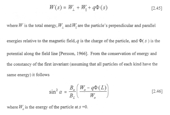
Figure 2.12 Schematic diagram of the simple geometry assumed for a parallel electric field in this analysis [Stern, 1981].

Equation [2.46] illustrates how the mirror points of ions and electrons are affected in different ways. For the parallel electric field shown in Figure 2.12 the ion mirror point is shifted away from the loss region, whereas the electron mirror point is pushed further in widening the loss cone. As an example, consider a 100 keV electron that mirrors at point P in Figure 2.13a. If the magnetic field intensity at P is 1000 nT and the magnetic field at the equator point O is 100 nT, in the absence of a parallel electric field, the pitch angle at the equator is 18°. If the magnetic field intensity at the loss edge is 1100 nT (point Q) the loss cone angle is 17.5°. For this situation, the particle’s mirror point is outside the loss region. However, if there is a potential difference between points O and M of 5040 Volts and if the distance is Δs=5 R_E, the electric field is then 1.68 10^-4 V/m . Then a particle at O with a pitch angle of 18° will not mirror until it reaches a magnetic field intensity of 1100 which is the within the loss region. The opposite will happen to an ion of the same energy (Figure 2.13b), where the mirror point is brought out of the loss region.

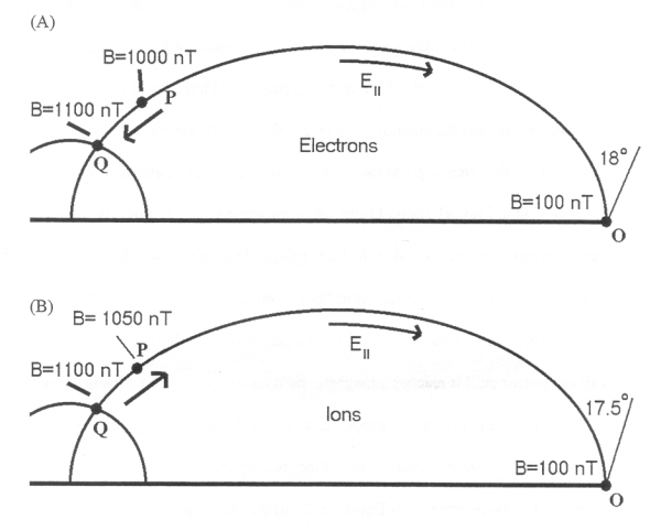Figure 2.13 (A) Mirroring geometry for electrons in the presence of a parallel electric field E||. A 100 keV electron with an equatorial pitch angle of 18° will mirror outside the loss region. The presence of a potential difference of 5 keV shifts the mirror point to the loss region. (B) Mirroring geometry for ions in the presence of a parallel electric field E||. A 100 keV ion with an equatorial pitch angle of 17.5° will mirror at the loss region.  The presence of a potential difference of 5 keV shifts the mirror away from the loss region.

It can also be inferred from Equation [2.46] that particles with different energies have their mirror points shifted in different amounts. Using the parameters of the example in the previous paragraph we will compare the amount of shift of two different electrons with 100 and 200 keV energies. The mirror point magnetic field intensity of a 100 keV electron was found to be 1100 nT in this situation, shifted from 1000 nT. A 200 keV electron will mirror at 1070 nT field which lies outside the loss region. Higher energy electrons are then shifted less than low energy electrons.

It could be argued that the parallel electric field sustained by a quasi-neutral equilibrium is the result of the unequal and anisotropic pitch angle distribution of magnetically trapped radiation and that as such particles are scattered by collisions and by convective plasma processes and become increasingly isotropic and maxwellian, such an E_|| would rapidly decay. One might consider the situation, in principle, where there is a difference in the electron (f_e) and ion (f_i) distribution functions without any continuous injection of new particles, and such an E_|| would eventually wash itself out by the balancing of f_e and f_i [Stern, 1981]. However, if the loss cone is continually refilled by convection, as in reality, the E_|| can maintain itself.

2.5.2 Corotational Electric Field

A rotating conducting body with a magnetic field produces an EMF according to

where Ω is the angular frequency of the rotating body, and r is the position where B(r) is measured [Cravens, 1997; Parks, 1991]. Equation [2.48] is the corotational electric field which adds a component of drift to equation [2.16]:

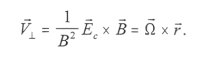
Equation [2.49] is charge independent, so both species of charged particle corotate with the rotating body in the same manner at the same velocity. For the Earth, the corotational electric field points inward at the equatorial plane. For Jupiter, it points radially outward.

Now that single particle theory has been covered, it is time to outline the particle detector and spacecraft that will detect these particles. Chapter 3 presents a detailed description of the EPD instrument, passbands and collimator acceptance angles. The second half of Chapter 3 details the pertinent coordinate systems, JSII (1965), GSI, GSII, spacecraft, and magnetic field coordinates.

Next: Chapter 3 Instrument Characteristics and Coordinate Systems

Return to dissertation table of contents page.

Return to main Galileo Table of Contents Page.
Return to Fundamental Technologies Home Page.

QUICK FACTS

RELATED LINKS