


Investigation of the Magnetosphere of Ganymede with Galileo's Energetic Particle Detector
Ph.D. dissertation by Shawn M. Stone, University of Kansas,
1999.
Copyright 1999 by Shawn M. Stone. Used with permission.
4.3 Modeling of External Sources: Magnetopause and Tail Fields
As was discussed in Chapter 1, the solar wind plasma impacts the magnetic field of the Earth, compressing it until a balance in pressure is achieved between the plasma pressure of the solar wind and the magnetic pressure of the Earth’s magnetic field. A magnetopause boundary forms, confining the magnetic field of the Earth from the interplanetary magnetic field. A tail field also results from currents that are induced when the solar wind plasma sweeps down the magnetosphere of the Earth.
The modeling of the Earth’s dayside magnetosphere has been approached in two ways. The first, and least desirable, is the method of an image dipole with variable position and strength to model the magnetopause boundary [Hones, 1963]. The second, more self-consistent, method is the boundary surface model which uses the external expansion in Equation [4.4] to construct a magnetopause field configuration [Mead, 1964; Choe et al., 1973; Choe and Beard,1974a]. The second method has also been applied to the tail field of the Earth [Choe and Beard, 1974b; Beard 1979].
4.3.1 Multipole Model of the Earth's Magnetopause Field
The magnetic field of the Earth is assumed to be the vector sum of Earth’s internal dipole Bd and the external field caused by the surface currents on the magnetopause boundary Bs. The total field is, then, in a system where the Z axis is the geographic north pole of the Earth and the X axis points in the anti-solar wind direction (towards the sun), in spherical coordinates
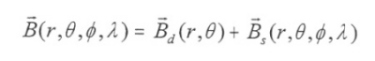 |
[4.7] |
where λ is the dipole tilt angle [Choe and Beard, 1974a].
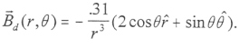
The dipole field expressed in gauss and r measured in Earth radii is
|
|
[4.8] |
The external field contribution depends on the surface current and the shape of the boundary. The currents on these surfaces are integrated using the Biot-Savart integral to obtain their contribution to the field at r:
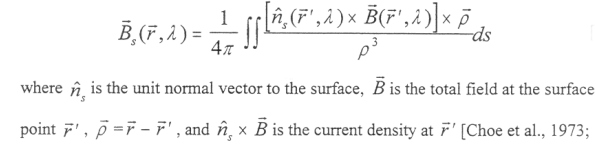 |
[4.9] |
Choe and Beard, 1974a], as illustrated in Figure [4.2].
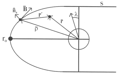 |
Figure 4.2 Schematic of the geometry required to integrate Equation [4.9]. The magnetic field contribution at r, from the surface currents at ρ, is obtained from the integration of the Biot-Savart integral along the surface S. |
The solution to Equation [4.9] is rather computationally complex. It begins by specifying an initial surface according to Mead and Beard [1964], and the field from the currents flowing on this first surface is calculated. This field is then used to improve the first surface configuration, and the process is repeated iteratively. It was found that after 9 iterations there was no more significant improvement in Bs [Choe et al., 1973; Choe and Beard, 1974a]. Since the magnetic field is assumed in this calculation to be irrotational inside the magnetosphere, the surface current field Bs can be expressed in terms of the external scalar potential expansion of Equation [4.4].
Using arguments of symmetry, the sin(mΦ) terms drop out [Choe et al., 1973], and Bs becomes
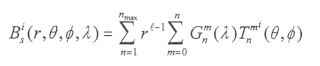 |
[4.10] |
where i=(1,2,3) corresponding to the three spherical coordinates r, θ, and Φ. The Tnmi terms depend on component
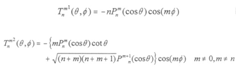 |
[4.11] [4.12] |
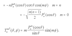 |
[4.13] |
Equation [4.10] can be expressed in terms of the sub-solar point ro (or offset distance) which is the point of pressure balance:
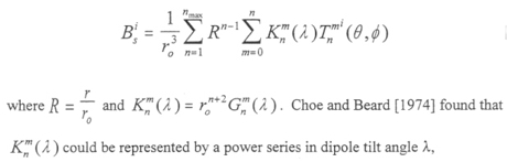 |
[4.14] |
|
|
[4.15] |
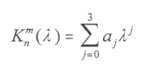
where aj=0 if n+m+j is odd from symmetry of the spherical harmonics. The coefficients Knm(λ) are calculated by a least squares fitting routine using 688 magnetic field values measured in the dayside magnetosphere [Choe et al., 1973; Choe and Beard, 1974a]. Table 4.2 shows these values up to nmax=2, but the coefficients up to nmax =7 can be found in Choe and Beard [1975].
Table 4.2 The coefficients aj in the series expansion of the spherical harmonic coefficients
Knm(λ), of the scalar magnetic potential for the magnetopause field up to nmax=2 [Choe and Beard, 1975].
| n | m | a0 | a1 | a2 | a3 |
| 1 | 0 | -.20105 | --- | -.00721 | --- |
| 1 | 1 | --- | -.06822 | --- | .04967 |
| 2 | 0 | --- | -.11839 | --- | .01976 |
| 2 | 1 | -.09232 | --- | .03050 | --- |
| 2 | 2 | --- | .01319 | --- | -.02192 |
Next: 4.3.2 Multipole Model of the Earth's Magnetotail Field
Return to dissertation table of contents page.
Return to main
Galileo Table of Contents Page.
Return to Fundamental
Technologies Home Page.
Updated 8/23/19, Cameron Crane
QUICK FACTS
Mission Duration: Galileo was planned to have a mission duration of around 8 years, but was kept in operation for 13 years, 11 months, and 3 days, until it was destroyed in a controlled impact with Jupiter on September 21, 2003.
Destination: Galileo's destination was Jupiter and its moons, which it orbitted for 7 years, 9 months, and 13 days.