


Investigation of the Magnetosphere of Ganymede with Galileo's Energetic Particle Detector
Ph.D. dissertation by Shawn M. Stone, University of Kansas,
1999.
Copyright 1999 by Shawn M. Stone. Used with permission.
4.8 Ganymede Field: Construction of Model 2
Model 2 consists of three field contributions: the uniform Jovian background within a radius of 10 Rg, the internal multipole field model of Ganymede, and the magnetopause and tail field from the external currents. The background field is based on the first 100 magnetic field points prior to the inbound magnetopause crossing at G2 and G7. These points are statistically averaged, and the mean and standard deviation are shown in Table 4.7. As in model 1, this background field is removed from the magnetic field data at the spacecraft before fitting. The internal field of Ganymede is modeled as a multipole in GSII coordinates up to nmax=2. The external sources consist of the model of the Earth's field to order nmax=2 scaled down by a factor of κ1 and κ2 for the tail and a factor of γ1 and γ2 for the magnetopause. The scaling factors used in the fitting of the magnetosphere of Mercury were predetermined from the different properties of the solar wind at the radius of Mercury from those at Earth. Also included in the model is the possible aberration of the magnetosphere's axis by an angle α about the GSII x axis and an angle β about the GSII z axis. This gives a total of 14 parameters to determine.
Table 4.7 The mean and standard deviation of the first 100 magnetic field components in GSII Cartesian coordinates. The data points are in 6s resolution.
| (Encounter) Component |
mean (nT) | Standard Deviation (nT) |
| (G2) Bx | -63.74 | ą4.40 |
| (G2) By | -26.05 | ą2.85 |
| (G2) Bz | -90.17 | ą1.70 |
| (G7) Bx | 66.85 | ą4.10 |
| (G7) By | 1.82 | ą2.64 |
| (G7) Bz | -77.35 | ą0.53 |
4.8.1 Setting Up the Equations and the Down Hill Simplex Method
The total field measured as the spacecraft passes through the magnetosphere of Ganymede is comprised of the field internal to the magnetospheric boundary BIM and the field external to the magnetospheric boundary BEM:
|
Btotal = BIM+BEM |
[4.28] |
where
|
BIM = BGanymede+BTail+BMagnetopause |
[4.29] |
Prior to the crossing of the magnetopause, the spacecraft is measuring the Jovian background field, since the magnetopause currents shield the external field from the internal. Once the spacecraft crosses the magnetopause, the internal field essentially "turns on" as shown in Figures 1.13 to 1.17, where the internal field due to Ganymede and the external sources of the magnetopause and tail are felt.
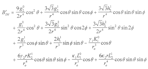
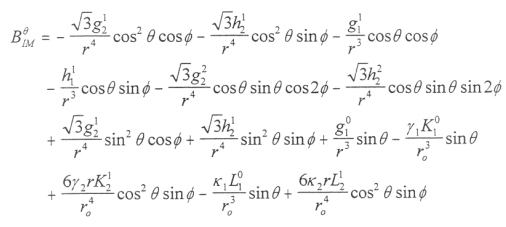
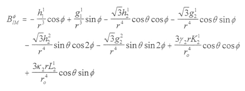
The first part of the procedure to define a magnetospheric model begins with the modeling of the internal field structure. From Equation [4.7] and Equations [4.10] through [4.14] to nmax=2, realizing that the Φ -->Φ+π/2 for the K and L terms to correctly adapt the Earth magnetopause and tail field configuration, gives by
 |
[4.30] |
 |
[4.31] |
 |
[4.32] |
component for the field internal to the boundary where K10, K21, L10, and L21 are the coefficients for the multipole model of the Earth given in Tables 4.2 and 4.3. The scaling factors γ1, γ2 and κ1, κ2 resize the magnetosphere of the Earth down to that of Ganymede based on the fitting procedure. The offset distance of the magnetopause is taken as 2.0 Rg.
The data set used to constrain the parameters of the internal multipole of Ganymede and the state of the magnetopause and tail field in Equations [4.30] through [4.32] is the G2 data set in GSII coordinates. This consists of 327 points between the inbound crossing (18:50:52) and the outbound crossing (19:22:31). The state of the magnetopause and tail field are thus determined for G2 in this case. The method used to fit Equations [4.30] through [4.32] is the down hill simplex method [Press et al., 1986] for the minimization of a function of more than one independent parameter, 12 in this case. The function to be minimized is constructed from the internal field components
|
|
[4.34] |
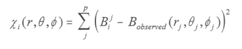
where i represents the components in spherical coordinates and the summation is over the p=327 data points. The results of the minimization are shown for G2 in Table 4.8 with standard deviations.
Table 4.8 Coefficients resulting from the minimization of Equation [4.33] for G2 for r0=2.0 Rg. The coefficients are reported in nT.
| G2 Coefficients |
Mean (nT) |
RMS Error |
| g10 | -715.56 | .80 |
| g11 | -66.82 | .46 |
| g20 | 36.32 | .53 |
| g21 | 102.42 | .35 |
| g22 | 43.15 | .50 |
| h11 | -305.08 | .65 |
| h21 | 202.89 | .60 |
| h22 | 33.98 | .54 |
| γ1 | -.01926 | .00026 |
| γ2 | .01245 | .00131 |
| κ1 | -.13470 | .00028 |
| κ2 | -.09561 | .00143 |
It is assumed at this point that the internal field is given by the internal coefficients in Table 4.8, and that the external coefficients are based on the plasma and field properties during the G2 encounter on this internal field. The parameters of the G7 field are then ascertained from the internal field given in Table 4.8, but the magnetopause and tail scale factors are refit as in the G2 procedure along with r0 as a fit parameter. The offset distance r0 was stepped in increments of .1 Rg, and Equation [4.33] was minimized at each step for 356 points between the inbound crossing (07:00:20) and the outbound crossing (07:36:00).
|
χTotal = χr + χθ + χΦ |
[4.33] |
When a minimum in Equation [4.33] was attained at ro=2.6, the procedure was halted. The results of this fit are given in Table 4.9. Figures 4.15 through 4.18 show each component of the magnetic field in GSII spherical coordinates for the G2 and G7 encounters. The field tracings are shown in Figures 4.19 to 4.26 and the determination of the magnetopause boundary is discussed in the next section.
Table 4.9 Coefficients for G7 resulting from the minimization of Equation [4.33] with the internal multipole model of Ganymede specified from Table 4.8.
| G7 Coefficients |
Mean |
RMS Error |
| γ1 | -.01527 nT | ą0.00029 nT |
| γ2 | .00911 nT | ą0.00174 nT |
| κ1 | -.09860 nT | ą0.00055 nT |
| κ2 | -.06998 nT | ą0.00295 nT |
| ro | 2.6 Rg | ą0.1 nT |
Next: 4.8.2 Solving and Mapping the Boundary
Return to dissertation table of contents page.
Return to main
Galileo Table of Contents Page.
Return to Fundamental
Technologies Home Page.
Updated 8/23/19, Cameron Crane
QUICK FACTS
Mission Duration: Galileo was planned to have a mission duration of around 8 years, but was kept in operation for 13 years, 11 months, and 3 days, until it was destroyed in a controlled impact with Jupiter on September 21, 2003.
Destination: Galileo's destination was Jupiter and its moons, which it orbitted for 7 years, 9 months, and 13 days.