Investigation of the Magnetosphere of Ganymede with Galileo's Energetic Particle Detector

Ph.D. dissertation by Shawn M. Stone, University of Kansas, 1999.

Copyright 1999 by Shawn M. Stone.  Used with permission.

5.2 Time Reversed Particle Tracing

Central to the simulation is the numerical integration of the Lorentz force equation. For a charged particle in the presence of both electric and magnetic fields the six equations of state for a particle of mass m_s and charge q_s in a Cartesian coordinate system are

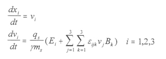
where x_i is position, n_i is velocity, E_i is the electric field, B_i is the magnetic field, and g is the relativistic correction factor. Given the initial conditions x_o and n_o the state of the particle at earlier times can be calculated.

Care must be taken in trying to visualize a dynamic system under time reversal. The Lorentz force equation is symmetric under time reversal, which means taking

gives back the same Lorentz equation

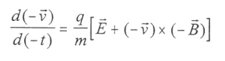
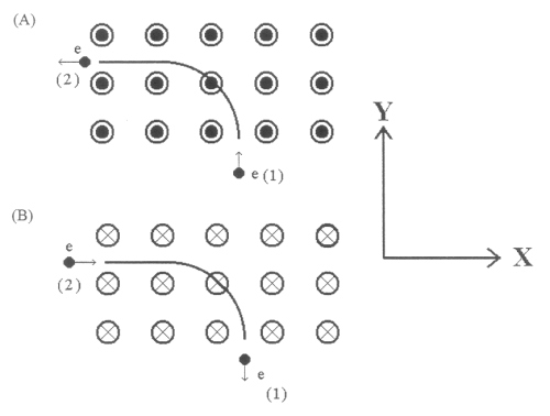
since the negatives cancel each other out. This symmetry ensures that conservation of energy is maintained. However, when one is tracing particles back in time, the particle must retrace its path. Consider the situation in Figure 5.3a, where an electron at point 1 is being sent into a uniform magnetic field. Its velocity points in the +y direction and its trajectory is bent to the -x direction until it leaves the field region at point 2. Under time reversal (Figure 5.3b) the velocity at point 2 is reversed and the magnetic field is now into the page. If time is now considered to flow positively in the other direction, the particle retraces its path until it reaches point 1 (t is not considered to go to -t).

Figure 5.3. (A) Diagram of an electron entering a region of uniform magnetic field (pointed out of the page) at point 1. Its trajectory is bent from the y direction to the -x direction to point 2. (B) Diagram of the same electron under time reversal. The magnetic field is into the page and the electron’s velocity vector is reversed in the x direction. The electron then retraces its path, moving now from point 2 to point 1 under time reversal.

5.2.1 Numerical Integration of the Lorentz Force Equation

Due to the complicated magnetic field geometry and possible presence of electric fields Equation [5.3] must be solved numerically. Particle_Follow uses the method of Bulirsch-Stoer which is thought to be the best known way to obtain high accuracy solutions to ordinary differential equations with a minimum amount of computational effort [Press et al., 1986]. Cast in difference form, on a time mesh, Equation [5.3] becomes [Potter, 1976]

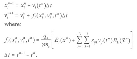[5.6]

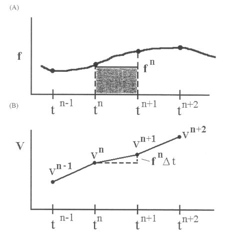
Typical numerical integration schemes such as Euler or Runge-Kutta integrate on the time mesh in discrete steps Dt, where Dt needs to be small in order for the solution to remain stable. Figure 5.4 illustrates the discrete time step integration of these methods for the velocity component of Equation [5.6].

Figure 5.4 (A) The state function f(vⁿ, xⁿ, tⁿ)=fⁿ evaluated on a time mesh at tⁿ. (B) The area under the f curve (fⁿDt) is the amount of the change in velocity from tⁿ to tⁿ⁺¹.

The Bulirsch-Stoer algorithm is based on the scheme of Richardson's approach to the limit using rational function extrapolation [Stoer and Bulirsch, 1980]. This approach is unique in the sense that instead of trying to take the smallest step possible, it takes the largest step possible. The major jump in logic of Richardson’s approach is to consider the final answer of the numerical calculation as an analytic function f(u,h) of an adjustable step size h=H/n where u(x,v) is the state of the particle, n is the number of step subdivisions (n=2,4,6,8, .....), and H is an arbitrarily large step size defined by the user. It is not important for the step size to be small enough for the accuracy that is desired because when enough is known about the function, it is fit to some analytic form, and then extrapolated to the ideal step size h=0.

Functions are commonly fit with a power series, but these have a limited radius of convergence out only to the first pole in the complex plane. Rational function fits can remain good approximations to the analytic functions even after the various terms in powers of h all have comparable magnitude. This means that h can be so large as to make the word “order” meaningless. The parameter space u is then integrated by h steps (first 2 steps, then 4, then 8, etc.) building f(u) as a function of h; see Figure 5.5. At each step the error is estimated and the algorithm stops when the desired error estimate is achieved. The resulting function is fit using a series of rational functions, and this function is then evaluated at a step size of h=0, thus taking an infinite number of steps to reach the solution f(u,h=0). The state of the particle is then evaluated at t+H. In this simulation, the choice of H depends on the gyroperiod of the particle: H=t_i/10 for ions, and H=t_e for electrons.

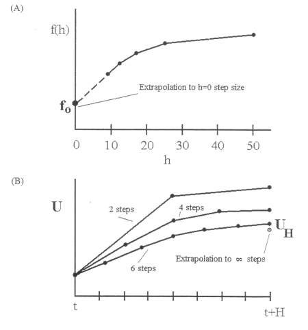Figure 5.5 (A) The function f(u,h) is evaluated as a function of step size, where H=100s to start. (B) The state of the particle is simultaneously evaluated at t+H/n, where n=2 steps, 4 steps, and 6 steps, etc. (h=H/n). UH represents the real value of the state of the particle at t+H if the step size is infinitesimally small h-->0 (an infinite number of steps). The series of points for f at these samples gives an idea of the form of f with respect to h by the fitting of f to a series of rational functions. When the simulation reaches the desired theoretical error estimate, the fitted function f is evaluated at h=0, giving UH(t+H).

Next: 5.2.2 Trace Criteria

Return to dissertation table of contents page.

Return to main Galileo Table of Contents Page.
Return to Fundamental Technologies Home Page.

QUICK FACTS

RELATED LINKS