Investigation of the Magnetosphere of Ganymede with Galileo's Energetic Particle Detector

Ph.D. dissertation by Shawn M. Stone, University of Kansas, 1999.

Copyright 1999 by Shawn M. Stone.  Used with permission.

5.6 Stepping Through the Encounter: Constructing the Simulated Count Rate

The entire process of calculating the initial conditions of the particles and then following them back in time through the magnetosphere of Ganymede is handled by Particle_Follow. A flow chart illustrating this process is shown in Figure 5.10. As was discussed in section 5.1, EphemerisGen processes the rate file containing the right ascension and declination angles of the spin axis in J1950 and the motor and sector positions, along with information contained in the SPICE kernels, to calculate the encounter geometry and EPD look directions in GSII coordinates. This information is contained in a data file, G2in1.dat for instance (the G2 encounter), where each record contains the necessary ephemeris information to calculate the initial conditions of the particle. Also, supplied to Particle_Follow is an ASCII file with the magnetic field vectors measured by the magnetometer for the purpose of calculating the pitch and phases used in the force pitch and phase mode.

Figure 5.10 Flow chart of the Particle_Follow program (within the dashed lines).  The ephemeris information needed to obtain initial conditions for the time reversed trajectories is provided by EphemerisGen, which has a record for each look direction contained in G2in1.dat for the G2 encounter. This file, along with the actual magnetic field vectors measured along the trajectory of Galileo (G2in2.dat) and a script file (run_file.s) that contains specific information to control the encounter, are provided to EncounterDriver.  The EncounterDriver reads the records from the input files and breaks them up into 39 initial conditions to be traced.  IntegrationDriver runs the reversed time following of the particles through the magnetosphere of Ganymede using ODEint, Bsstep, MMid, and RzExtr to move the particle from t to t+H. When the boundary conditions are exceeded or the particle impacts Ganymede, control is passed from IntegrationDriver back to EncounterDriver where the result is saved in a file cataloging the run. The next look direction is read, and the process continues. 

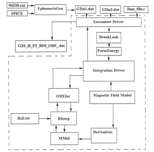
The EncounterDriver reads this information a record at a time; the first record is encounter index 1, the second record is encounter index 2, and so on. These indexes can be specified in a run_file in order to narrow the run to a single feature if needed or even a single trajectory if the index ranges are known. Also in the run_file are the parameters for the run, such as energy channel, trace criteria, strength of parallel electric fields, scattering coefficient, and whether to run in extended bounce or single shot mode. The look direction is then divided into 13 sub-look directions and the passband of the energy detector specified is divided into 3 energies. This information is then converted into 39 initial velocities, and, along with the position of the spacecraft, these are passed one at a time to the IntegrationDriver.

The IntegrationDriver is the heart of Particle_Follow, keeping track of where the particle is at each integration step, checking to see where it is and how long it has been integrated. It adjusts the step size H as needed, stepping through the magnetosphere a little bit at a time, by passing control to the ordinary differential equation integrator ODEint. ODEint breaks H up into n sub-steps as specified in section 5.2.1, and implements the Bulirsch-Stoer method through BSstep (estimates the error of each successive step), MMid (implements the modified mid point method), and RzExtr (which uses rational functions to fit the resulting solution as a function of step size). When the solution falls within the accuracy dialed in (which for this work is 1 x 10-6) ODEint passes control back to IntegrationDriver with the new state of the particle.

There are several quantities that are kept track of, along with the position and velocity, as the particle is stepped through the magnetosphere of Ganymede: the total trace time, the maximum and minimum values of the magnetic field and first invariant µ, the final position of the particle, and the pitch and phase angles of the particle. When the particle hits Ganymede or the trace criteria have forced an exit, control passes back to EncounterDriver, which stores the result of the run in an output file. The output files are labeled according to the encounter such as the example shown in Figure 5.10, G2s_B_F2_B10_1569.dat, which stands for G2 encounter model 2 energy channel F2 extended bounce mode (S=10 Rg) encounter index 1569. This means a distribution of particles with energies distributed within the F2 passband were traced back in time in extended bounce mode with model 2 only for a feature that starts at encounter index 1569. From this point on, all features will be referred to by encounter, and the UT time of the first sector of the spin (G2,G7): (hour)(minute)(second); encounter index 1569 referring to feature G2:191051.

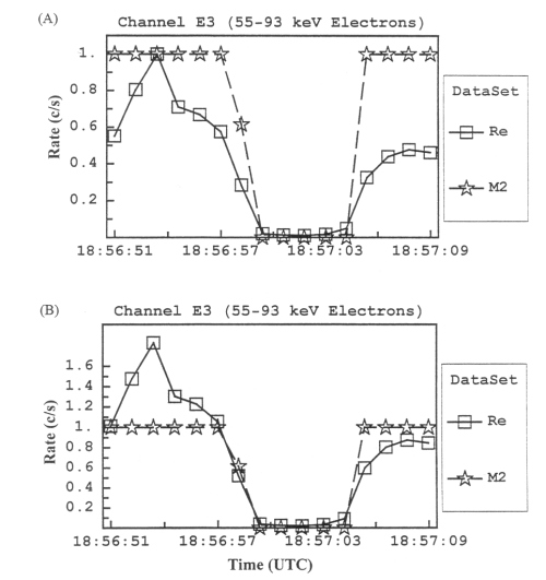
The goal of the simulation as it traces these particles back in time from the EPD instrument is to construct a simulated rate profile to compare to the actual one measured. Particles that hit Ganymede are removed from the distribution of n particles (39 or 65 as discussed above), and particles that leave the boundary sphere S or run beyond the time limit are not lost. In this fashion, a simulated count rate can be constructed. To compare the simulated rates (with a max count of 39) with the real rate profiles which can have counts out to 105, a normalization method must be implemented.

Figure 5.11 shows two rate profile comparisons between the real data and model M2 for feature G2:185651 for two normalizations. Figure 5.11a shows an example of normalization to the maximum rate of the spin. This method is prone to random rate fluctuations and sources, which are not included in the simulation. It was decided to use a normalization scheme of normalizing to the rate at a pitch angle of 90° since this probably represents the local steady state count rate. Figure 5.11b shows the same feature normalized to 90° pitch, which brings the simulated and real to a realistic comparison. Many of these results will be presented in the following two chapters.

Figure 5.11 Rate profiles of feature G2:185651. In order to compare the real data (Re) with the simulated (in this case from model M2) the two sets must be normalized. (A) Normalization to the maximum rate in a spin. This type of normalization can be tricky, since it is prone to sources like the one shown here. (B) Normalization to the rate near 90º of pitch in a spin. Particles at pitches of 90º tend to represent the closest estimate of the steady state background rate since they tend to remain in the local region. The result is a better comparison between the real measured data and the model data.

Next: Chapter 6 Time-Reversed Particle results: G2 Encounter

Return to dissertation table of contents page.

Return to main Galileo Table of Contents Page.
Return to Fundamental Technologies Home Page.

QUICK FACTS

RELATED LINKS