


Investigation of the Magnetosphere of Ganymede with Galileo's Energetic Particle Detector
Ph.D. dissertation by Shawn M. Stone, University of Kansas,
1999.
Copyright 1999 by Shawn M. Stone. Used with permission.
6.2.1 Ion Results
The time reversed particle following of charged particles in the inbound phase for ions revealed absorption signatures with the same quality as the features observed in the real data (Figure 6.8). This will give a unique perspective as to the origins of these seemingly random features since Particle_Follow (Chapter 5) allows a detailed analysis of each of the trajectories that make the simulated count rate. Figure 6.10 shows feature G2-18:43:11 for channel A4 model M1. A depression can be seen in the simulated rate at about 18:43:26 UT. This may seem strange since an ion in a 100 nT field with an energy of 400 keV (Channel A4) has a gyroradius of about .33 Rg. (Figure 6.6 shows that Galileo is about 3 Rg from the center of Ganymede.)
Figure 6.10 (A) Simulated M1 and real (Re) rate profile for feature G2-18:43:11 of Channel A4 normalized to 90º of pitch. The arrow points to a data point that will be broken down for further analysis. (B) The pitch and phase angles are computed from the look direction of the EPD detector and the appropriate magnetic field vector R for real and S for simulated.
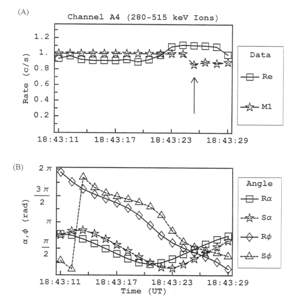
To investigate the origins of this signature a data point in the simulated feature is chosen such as the one indicated with an arrow in Figure 6.10. This particular point is constructed from the distribution of particles that were traced back in time through model M1. The distribution consists of particles with initial conditions obtained from the subdivision of the A4 pass band into 5 subenergies (319 keV, 358 keV, 400 keV, 437 keV, 476 keV) and 13 sublook directions giving a total of 69 individual trajectories. Figure 6.11 shows a collimator pitch and phase scatter plot for subenergy 400 keV. As can be immediately seen, this is not a loss cone feature. The impacts with Ganymede (shown by the filled in squares) are not ordered by pitch angle or phase. A detailed trace back for sublook 1 (miss) and sublook 5 (hit) is performed; figures 6.12 through 6.17 show the results for subenergy 400 keV sublook 1 for model M1 channel A4 whose significance is summarized in Table 6.1.
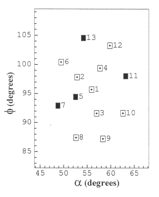 |
Figure 6.11 Collimator pitch and phase scatter plot for the sector pointed out in Figure 6.10 for M1 A4 18:43:11 subenergy 400 keV. The angles are in degrees. The filled in squares represent trajectories that intersected the surface of Ganymede and were absorbed. Open squares represent trajectories that missed. |
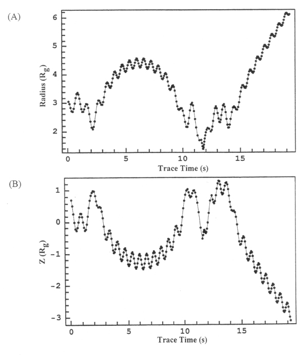 |
Figure 6.12 (A) Length of the radius vector from the center of Ganymede to the particle as a function of trace time in seconds for subenergy 400 keV sublook direction 1 for model 1 channel A4. Ten points comprise a gyroperiod. (B) The Z component of the particle position in GSII coordinates for subenergy 400 keV sublook direction 1 for model 1 channel A4. |
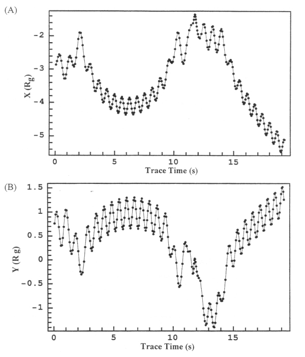 |
Figure 6.13 (A) The X component of the particle position in GSII coordinates for subenergy 400 keV sublook direction 1 for model 1 channel A4. (B) The Y component of the particle position in GSII coordinates for subenergy 400 keV sublook direction 1 for model 1 channel A4. |
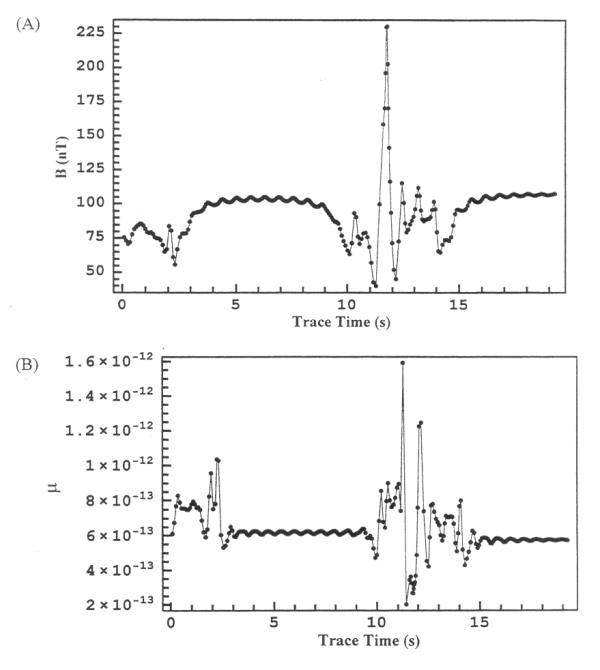 |
Figure 6.14 (A) Magnetic field at the location of the particle as a function of trace time for subenergy 400 keV sublook direction 1 for model 1 channel A4. (B) Magnetic moment at the location of the particle as a function of trace time for subenergy 400 keV sublook direction 1 for model 1 channel A4. |
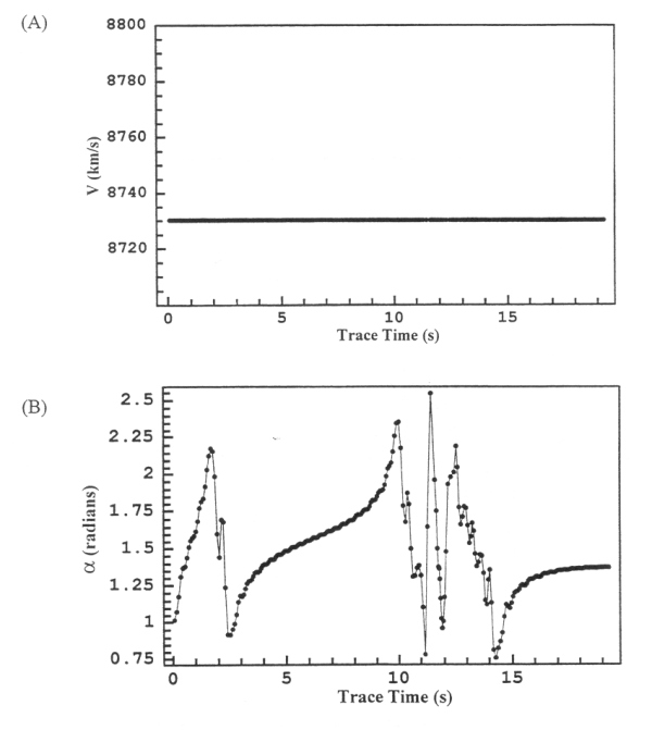 |
Figure 6.15 (A) Velocity of the particle as a function of trace time for subenergy 400 keV sublook direction 1 for model 1 channel A4. (B) Pitch angle of the particle as a function of trace time for subenergy 400 keV sublook direction 1 for model 1 channel A4. |
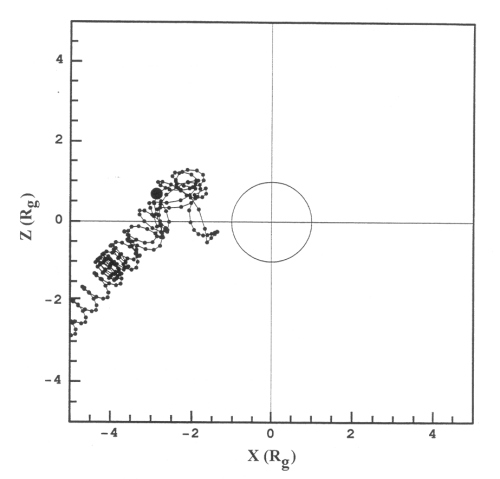 |
Figure 6.16 ZX projection of the trajectory for subenergy 400 keV sublook direction 1 for model 1 channel A4. |
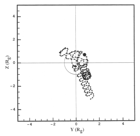 |
Figure 6.17 ZY projection of the trajectory for subenergy 400 keV sublook direction 1 for model 1 channel A4. |
Table 6.1 Summary of the time reversed particle trace presented in Figures 6.12 through 6.17 for subenergy 400 keV sublook direction 1 for model M1 channel A4.
| Figure | Information | Observation |
| 6.12 | (A) Radius of particle from Ganymede. (B) Z component of particle trajectory. | Null point slips (translation) can be seen at trace times of 2 s and 10 s. |
| 6.13 | (A) X component of particle trajectory. (B) Y component of particle trajectory. | Null point slips (translation) can be seen at trace times of 2 s and 10 s. |
| 6.14 | (A) Magnetic field sampled by the particle. (B) Magnetic moment sampled by the particle. | Null points in the field (dips toward zero field) can be seen at 2 s and 10 s. The magnetic moment external to these times can be seen to remain constant (gyro phased averaged). At these times, however, there is wild variation. |
| 6.15 | (A) Speed of the particle as it moves through its trajectory. (B) Pitch angle of the particle. | The speed of the particle (thus energy) is conserved even though the motion goes non-adiabatic at the null points. The pitch angle of the particle at the null points oscillates with the apparent magnetic field direction which is poorly defined within the null. |
| 6.16 | ZX projection of the trajectory of the particle. | It can be seen that when the particle is in a region of nominal field, the motion is translational. In regions of stronger field, the particle gyrates as expected. |
| 6.17 | ZY projection of the trajectory of the particle. | It can be seen that when the particle is in a region of nominal field, the motion is translational. In regions of stronger field, the particle gyrates as expected. |
The first important detail to notice is plainly seen in Figure 6.14a, which is a plot of the magnetic field as seen at the location of the particle versus simulated trace time. There are two points where the magnetic field dips towards zero: one at about 2 s and one starting at 10 s. The corresponding first invariant plot is shown in Figure 6.14b which shows sudden shifts at these times. Inspecting the radius from the center of Ganymede (Figure 6.12a) and the Cartesian components of the position in GSII (Figures 6.12b, 6.13a, and 6.13b) show a translating instead of gyrating motion. At first, this could be mistaken for numerical error, but an inspection of the speed of the particle during the entire trace shows it remains constant (Figure 6.15a). Also, Particle_Follow tags trajectories that violate the chosen accuracy (1x10⁻⁶) and these did not do so. Figure 6.15b shows the corresponding pitch angle of the particle. At the regions of low magnetic field, labeled from now on as null points, the pitch angle shifts randomly, since the vector direction of the magnetic field in the null point can be unpredictable.
Return to dissertation table of contents page.
Return to main
Galileo Table of Contents Page.
Return to Fundamental
Technologies Home Page.
Updated 8/23/19, Cameron Crane
QUICK FACTS
Mission Duration: Galileo was planned to have a mission duration of around 8 years, but was kept in operation for 13 years, 11 months, and 3 days, until it was destroyed in a controlled impact with Jupiter on September 21, 2003.
Destination: Galileo's destination was Jupiter and its moons, which it orbitted for 7 years, 9 months, and 13 days.