


Investigation of the Magnetosphere of Ganymede with Galileo's Energetic Particle Detector
Ph.D. dissertation by Shawn M. Stone, University of Kansas,
1999.
Copyright 1999 by Shawn M. Stone. Used with permission.
6.3.1 Feature G2-18:56:31 (continued)
The collimator pitch and phase scatter plot for this point extracted from model M2 is shown in Figure 6.76. Subenergy 74 keV was chosen. The look direction chosen for tracing is sublook direction 3 which has a pitch of 139° and a phase of 175°. The results of the trace are shown in figures 6.77 through 6.82 and are summarized in Table 6.9. In this case, the 74 keV electron can be seen to bounce out of the interaction region and then anti-corotate completely past Ganymede. It does not have a secondary interaction and then does not produce a loss cone in the anti-moon direction.
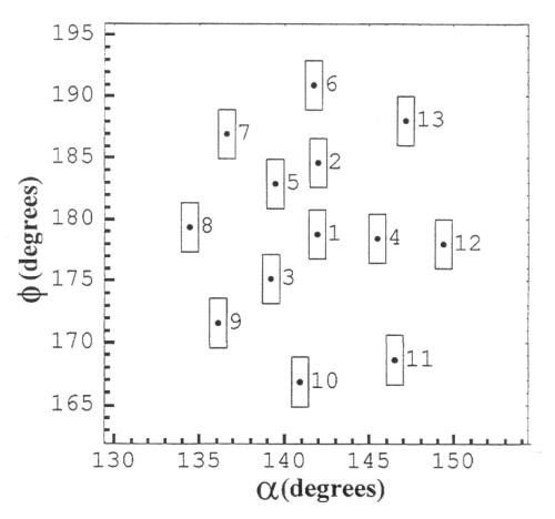 |
Figure 6.76 Collimator pitch and phase scatter plot for the sector pointed out in Figure 6.68 for M2 E3 G2-18:56:31 subenergy 74 keV. The angles are in degrees. The filled in squares represent trajectories that intersected the surface of Ganymede and were absorbed. Open squares are trajectories that missed. |
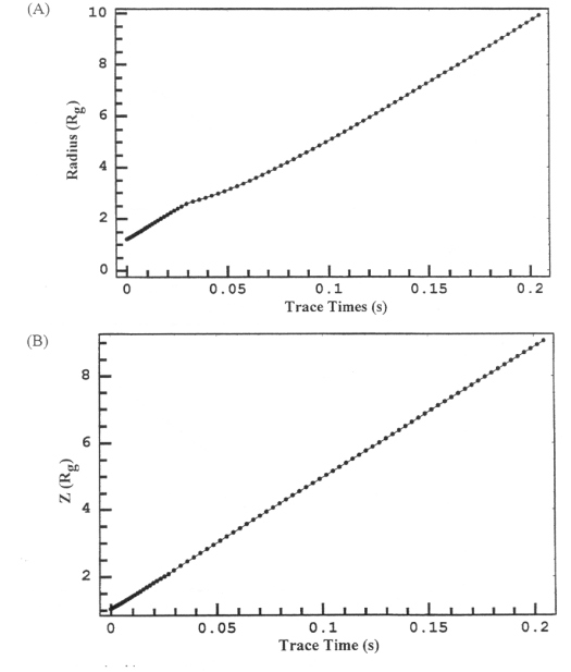 |
Figure 6.77 (A) Length of the radius vector from the center of Ganymede to the particle as a function of trace time in seconds for subenergy 74 keV sublook direction 3 for model M2 channel E3. (B) The Z component of the particle position in GSII coordinates for subenergy 74 keV sublook direction 3 for model M2 channel E3. |
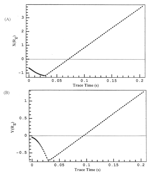 |
Figure 6.78 (A) The X component of the particle position in GSII coordinates for subenergy 74 keV sublook direction 3 for model M2 channel E3. (B) The Z component of the particle position in GSII coordinates for subenergy 74 keV sublook direction 3 for model M2 channel E3. |
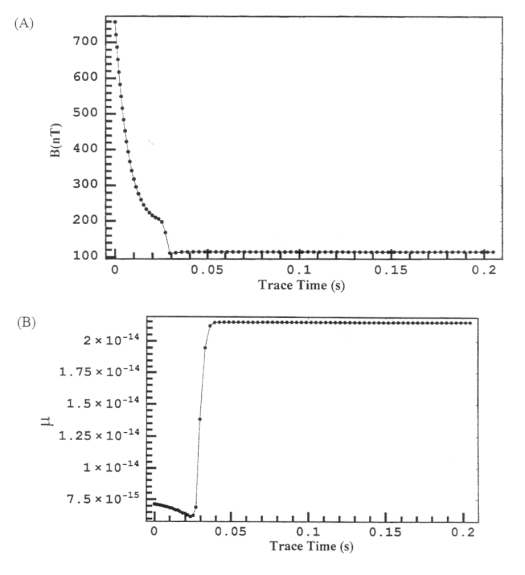 |
Figure 6.79 (A) Magnetic field at the location of the particle as a function of trace time for subenergy 74 keV sublook direction 3 for model M2 channel E3. (B) Magnetic moment at the location of the particle as a function of trace time for subenergy 74 keV sublook direction 3 for model M2 channel E3. |
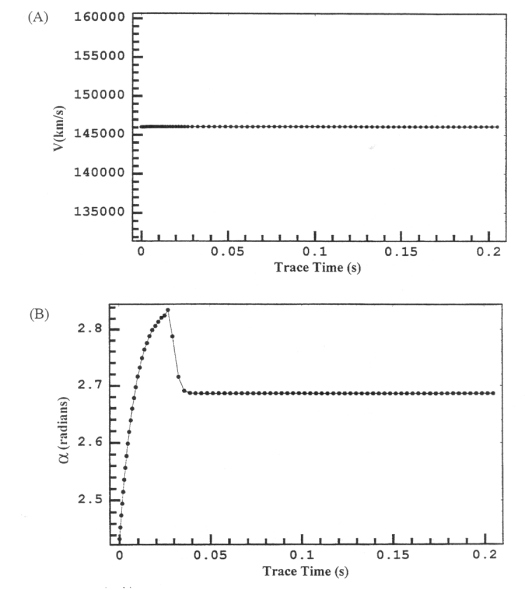 |
Figure 6.80 (A) Velocity of the particle as a function of trace time for subenergy 74 keV sublook direction 3 for model M2 channel E3. (B) Pitch angle of the particle as a function of trace time for subenergy 74 keV sublook direction 3 for model M2 channel E3. |
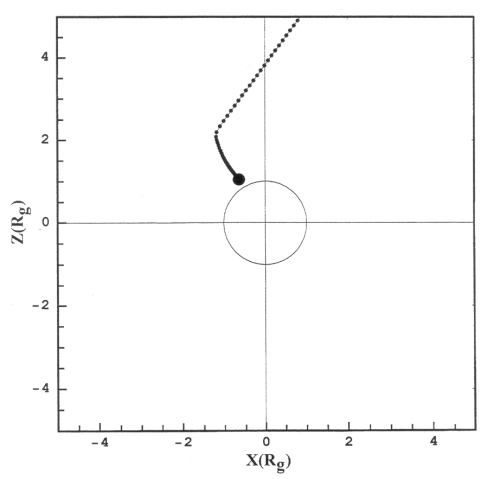 |
Figure 6.81 ZX projection of the trajectory for subenergy 74 keV sublook direction 3 for model M2 channel E3. |
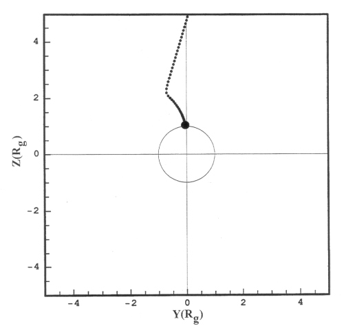 |
Figure 6.82 ZY projection of the trajectory for subenergy 74 keV sublook direction 3 for model M2 channel E3. |
Table 6.9 Summary of the time-reversed particle trace presented in Figures 6.77 through 6.82 for subenergy 74 keV sublook direction 3 for model M2 channel E3.
| Figure | Information | Observation |
| 6.77 | (A) Radius of particle from Ganymede. (B) Z component of particle trajectory. | It is easy to see from these two plots that the electron does not have a second interaction with Ganymede. |
| 6.78 | (A) X component of particle trajectory. (B) Z component of particle trajectory. | The internal magnetic field geometry can be seen to guide the electron in the corotation direction until it leaves the magnetosphere of Ganymede. |
| 6.79 | (A) Magnetic field sampled by the particle. (B) Magnetic moment sampled by the particle. | The magnetic field shows a smooth transition from the internal field of Ganymede to the external field. The electron doesn't have a secondary interaction with Ganymede. The magnetic moment varies smoothly across the boundary and remains constant. |
| 6.80 | (A) Speed of the particle as it moves through its trajectory. (B) Pitch angle of the particle. | The speed of the electron remains constant throughout the trajectory. The pitch angle decreases to 2.82 radians on the way out and transitions to 2.7 across the boundary. |
| 6.81 | ZX projection of the trajectory of the particle. | The electron is shown following the magnetic field line very closely. |
| 6.82 | ZY projection of the trajectory of the particle. | The electron follows the magnetic field geometry and can be seen to be guided in the anti-corotation direction on its way out. |
In the presentation of scattering to follow, not all rate profiles will be shown, but the results will be summarized in Figures like 6.83 and 6.84, and the remaining plots are presented in Appendix C and summarized in Table 6.10. These plots are produced from the correlation of the real rate profiles with those of the simulated as a function of scattering coefficient. The scattering coefficient that best matches the data produces the best correlation. In this case, for channel F2, a scattering coefficient of Daa=2x10⁻³ s-1 for model M1 and Daa=6x10⁻³ s-1 for model M2 produce the greatest degree of agreement. This will be done for each electron channel in the rest of the dissertation.
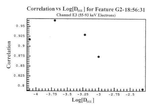 |
Figure 6.83 Correlation of feature G2-18:56:31 with simulated M1 data for varying values of Daa. This graph shows that the scattering coefficient with the highest correlation is Daa=2 x 10⁻³ s. |
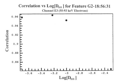 |
Figure 6.84 Correlation of feature G2-18:56:31 with simulated M2 data for varying values of Daa. This graph shows that the scattering coefficient with the highest correlation is Daa=6 x 10⁻³ s. |
Table 6.10 Summary of features of model M1 and M2 not included in the main body of the text for the closest approach portion of the G2 encounter. The corresponding graph is presented in Appendix C. The precise graph is indicated in the description column.
| Feature | Model | Description |
| G2-18:56:31 | M1 | Ion channels A2 and A6 fit the real data very well. The electron channel E1 seems to appear slightly before the observed feature, and with the addition of scattering in extended bounce mode an anti-moon loss cone is picked up. This anti-moon loss cone does not exist in the observed data. See Figures C15 to C19. |
| G2-18:56:31 | M2 | Ion channels A2 and A6 fit the real data very well. The electron channel E1 fits the observed data as well. With the addition of scattering in extended bounce mode an anti-moon loss is not picked up as observed in the real data. See Figures C20 to C24. |
| G2-18:58:31 | M1 | Ion channels A2 and A6 fit the real data very well. The electron channel E1 fits the observed loss cone as well. With the addition of scattering in extended bounce mode an anti-moon loss cone is picked up; however, it was only possible to match the feature somewhat. See Figures C25 to C29. |
| G2-18:58:31 | M2 | Ion channels A2 and A6 fit the real data very well. The electron channel E1 fits the observed loss cone as well. With the addition of scattering in extended bounce mode an anti-moon loss cone is picked up and the relative shape and depth is matched. See Figures C30 to C33. |
Next: 6.3.2 Feature G2-18:58:31
Return to dissertation table of contents page.
Return to main
Galileo Table of Contents Page.
Return to Fundamental
Technologies Home Page.
Updated 8/23/19, Cameron Crane
QUICK FACTS
Mission Duration: Galileo was planned to have a mission duration of around 8 years, but was kept in operation for 13 years, 11 months, and 3 days, until it was destroyed in a controlled impact with Jupiter on September 21, 2003.
Destination: Galileo's destination was Jupiter and its moons, which it orbitted for 7 years, 9 months, and 13 days.