


The Galileo Energetic Particles Detector
Galileo EPD Handbook
Chapter 1. Instrument Summary
Charged Particle Response of Magnetic Deflection System for Galileo Jupiter Orbiter (draft) (continued)
Methods of Calculation
We divided a detector surface into smaller sample areas, each measuring 0.08 x 0.08 cm2. The center of the sample area is used as an initial position called a sample point. Starting from a sample point on a detector, we chose uniformly distributed polar and azimuthal angles and approximately logarithmically spaced energies for the particles. The equations of motion (equations (1) and (2)) are solved numerically using a fourth-order predictor-corrector method in a time-reversed sense. Along a solved trajectory, every line segment is composed of two points (xi, yi, zi and xi+1, yi+1, zi+1). Each line segment was tested against all detector surfaces, the side surfaces, the aperture surfaces, and the channel surfaces in order to determine whether the trajectory passes the sensor or not. Each test is performed by examining if the intersection point of a line segment is inside or outside the boundaries of the surfaces as described in Figure 6.
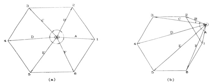 |
Figure 6. (a) The directions of A x B, B x C, C x D, D x E, E x F, and F x A remain unchanged; therefore the intersection point lies inside the polygon. (b) The directions of A x B and B x C are opposite; therefore the intersection point lies outside the polygon. |
By using this method, we can determine if a particle collides with the interior surfaces or goes through any of the detectors. This process can be repeated for the purpose of scanning different polar and azimuthal angles to form a set of trajectories of the particle. Then, for this starting point, the number of detected particles can be determined and the solid angle spanned by the set of trajectories can be computed. After examining all sample areas, the geometric factor for this energy and the detector can be obtained by using equation (11).
Figure 7 shows that an electron trajectory intersects with a detector segment in the coordinate system of the simulation. The polar and azimuthal angles are also shown for the calculation of the geometric factors. The geometric factor of detectors at a given energy is defined as follows:

where ΔA is the sample area and n is the number of sample areas. ΔΩ is the solid angle spanned by open trajectories. It also depends upon the energy of the particle and the number of detected particles (or the number of open trajectories).
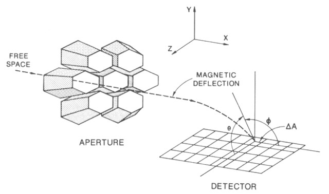 |
Figure 7. A segment of electron trajectory intersects with a detector. ΔA is the sample area on the detector and θand φ are the polar and azimuthal angles, respectively. |
For a particular energy of the particle at a starting point, the solid angle can be evaluated:

where Δθ and Δφ are the scanning angle intervals. Since we used 1° and in some cases 0.5° for Δθ or Δφ, the approximation is justified.
Next: Results of the Simulation
Return to Galileo EPD Handbook Table of Contents Page.
Return to main
Galileo Table of Contents Page.
Return to Fundamental
Technologies Home Page.
Updated 8/23/19, Cameron Crane
QUICK FACTS
Mission Duration: Galileo was planned to have a mission duration of around 8 years, but was kept in operation for 13 years, 11 months, and 3 days, until it was destroyed in a controlled impact with Jupiter on September 21, 2003.
Destination: Galileo's destination was Jupiter and its moons, which it orbitted for 7 years, 9 months, and 13 days.