The Galileo Energetic Particles Detector

Galileo EPD Handbook

Chapter 1. Instrument Summary

Charged Particle Response of Magnetic Deflection System for Galileo Jupiter Orbiter (draft) (continued)

Magnetic Field Model

The magnetic field is due to a uniform magnet lying in the x-y plane with its center at the origin; its integral form [7] is given by

where σ_M is the surface density of the magnetic pole strength. M is the magnetization, which is constant, and its direction is the same as the normal of the magnet. The factor M/c is converted to the normalization constant B₀ which was used to fit experimental values of the field.

We obtained this three-dimensional, analytic expression for B(x,y,z) by evaluating the integral [8]. Its components are given in equations (5), (6), and (7). From these expressions, we constructed a complete analytic expression for the field provided by both separate magnets. The experimental measurements of magnetic field strength are only available in the middle plane (z=0.0) where, because of the symmetry of the sensor, B_x=B_y=0 should vanish [9]. The two magnets are placed in a pattern: one at the left tilted counter-clockwise by an angle, the other tilted at the right clockwise by an angle of the same degree. For this arrangement, the expressions of both magnets require a coordinate rotation as well as a translation of the coordinate system. These transformations are given in equations (8), (9), and (10).

where a is the half-width of the magnet, l the half-length of the magnet, and B₀ the normalization constant of the magnetization.

The rotation of the coordinates for the left magnet is given by

the rotation of the coordinates for the right magnet by

and the translation of the coordinates for both magnets by

where y'₁ and z'₁ are for the left magnet, y'₂ and z'₂ are for the right magnet, d is the separation between the left and right magnets, ψ is the angle by which the magnets are tilted, and x₁, y₁, and z₁ are the distances shifted from the origin of the coordinates.

In addition, in order to simulate the actual measurements of the field, the two magnets are further divided into smaller pieces. For each of the smaller magnets, the rotation and translation were carried out. The magnetization values of all small magnets are obtained by normalizing the maximum field value from the experimental data. Figure 3 provides the distribution of the magnetizations of these magnets.

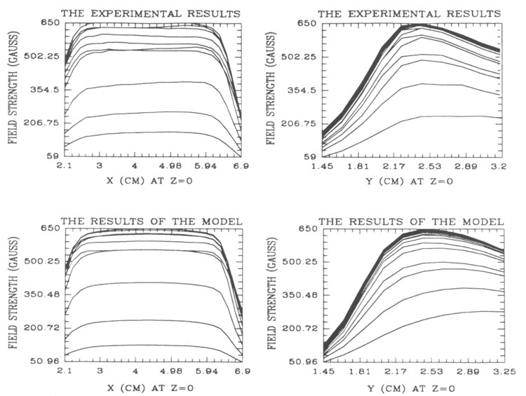Figure 3. Comparison between measurements and results of the model. Each curve corresponds to a different specific value of y (left) and x (right).

The superposition of these small magnets (both left and right) results in the total field strength and gives a good agreement with the experimental data inside the sensor (see Figure 3). The magnetic field lines are computed and projected on both the y-z and the x-z plane as given in Figure 4. These field lines converge to the fringes of the magnets. The contour plots in Figure 5 demonstrate the expected variation of the field and show the divergence, and the curl of the magnetic field vanishes inside the sensor. The results show that the edges of the magnets are highly magnetized and the field is stronger where the two magnets are closer. The numerical results of the magnetic field of the magnetic field and the parameters used in the simulation are provided elsewhere [10].

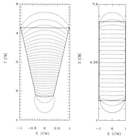	Figure 4. Projection of the magnetic field lines in the y-z plane at x=4.32 cm (left panel) and in the x-z plane at y=4.18 cm (right panel). The maximum field strength at z=0 is 650 G.
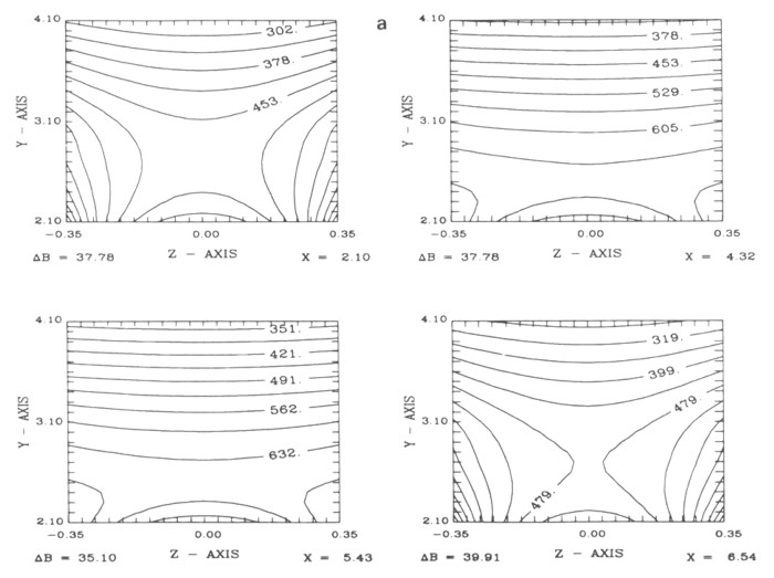	Figure 5a. Contour plots of the magnitude of the magnetic field.
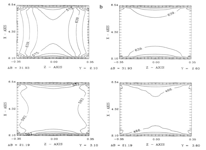	Figure 5b. Contour plots of the magnitude of the magnetic field.
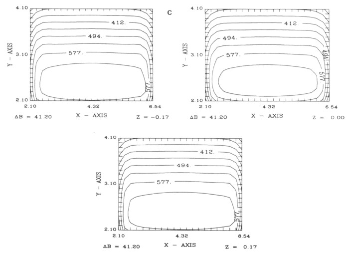	Figure 5c. Contour plots of the magnitude of the magnetic field.

Next: Methods of Calculation 

QUICK FACTS

RELATED LINKS