Investigation of the Magnetosphere of Ganymede with Galileo's Energetic Particle Detector

Ph.D. dissertation by Shawn M. Stone, University of Kansas, 1999.

Copyright 1999 by Shawn M. Stone.  Used with permission.

2.4 Pitch Angle Diffusion

Due to the conservation of the first adiabatic invariant, a charged particle whose pitch angle lies outside the loss cone is trapped. However, if there is a mechanism that somehow alters the pitch angle so that it lies within the loss cone (α<α_LC), the particle can be lost from the trapped distribution. This requires a mechanism that can operate on time scales smaller than a gyroperiod in order to violate the first invariant. The redistribution of particle pitch angles in a stochastic fashion resulting from such forces may be viewed as a diffusion process in pitch angle space [Kennel and Petschek, 1966; Roberts, 1969]. How pitch angle diffusion leads to trapped particle loss is shown schematically in Figure 2.9. As the particle bounces along the field line it can be scattered multiple times in a random walk, changing its energy and pitch angle. After several scattering events the particle can accumulate a Δα that puts it into the loss cone. There are several mechanisms that could facilitate this: charge exchange, atmospheric scattering of electrons, and wave-particle interactions [Roberts, 1969]. The section that follows presents a Fokker-Planck formalism that will be applied to wave-particle interactions but can be applied to any pitch angle scattering mechanism.

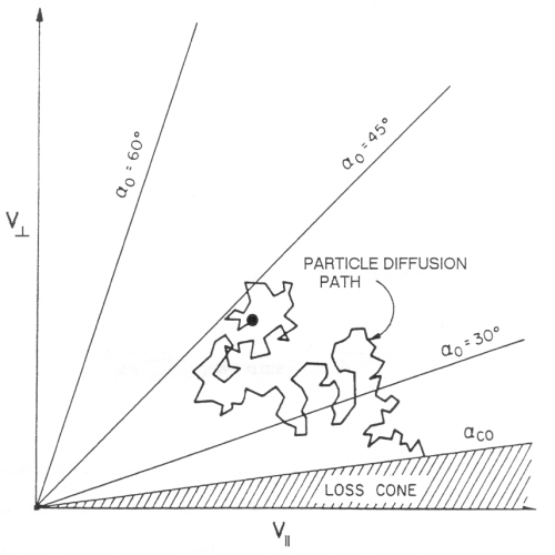Figure 2.9 Loss of a trapped particle by a random walk in velocity space into the pitch angle loss cone [Roberts, 1969].

2.4.1 Pitch Angle Diffusion Equation and Particle Lifetime

One example of wave-particle interaction is a stochastic process in which particles are scattered by whistler mode waves. If the mean velocity change is small, the distribution obeys the Fokker-Planck equation where Δα only changes and energy is conserved [Chandrasekhar, 1960]:

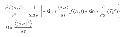[2.31]

Angular brackets denote an average over the fluctuation spectrum and Δt is the mean time step per wave collision [Kennel and Petschek, 1966]. The first term in the curly brackets is the average over fluctuations. In this case it is assumed that the change in pitch angle is evenly distributed about the mean, so <Δα>=0. The second term can then be differentiated to give

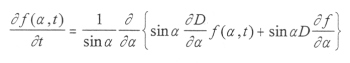
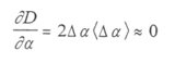
and recognizing that

yields the pitch angle diffusion equation

in the absence of sources.

Of course, without sources, the entire population of particles would eventually be scattered into the loss cone. Let us consider a steady state solution where particles are injected on a given velocity space-energy shell at flat pitches (α=π/2) on a given tube of force and diffuse in pitch angle until they reach the loss cone (α_LC ), so that loss and injection balance each other [Kennel,1969]. Equation [2.34] becomes

[2.35]

for pitch angles outside the loss cone α>α_LC where S is the source flux and

within the loss cone α<=α_LC [Kennel, 1969; Treumann and Baumjohann, 1997]. The loss term f/T_B assumes that the particles being lost leave the system in a scale time comparable to the bounce time that it takes to go from the equatorial plane to the loss region and α_o«1. In the case of trapped particles being lost to an atmospheric loss cone, this is the quarter bounce time for zero pitch-particles T_B. The solution to Equation [2.35] for f_e can be found in the treatment of Kennel [1969], who uses Green's functions, and is of the form

where <S(ν)> is the average of the injection source over pitch angle

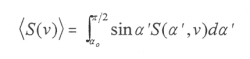
and h(α^o) is the pitch angle distribution function within the loss cone.

The arbitrary function H(α) must be determined from the boundary conditions. In order to do this, a form for D(α) must be assumed rather than solve Equation [2.36] for an arbitrary D(α). By assuming D(α)=D₀sinⁿα --> D₀αⁿ, h(0) is finite,

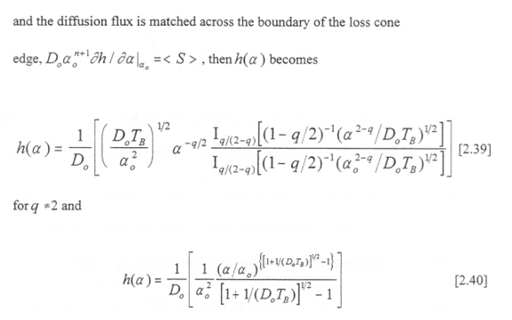
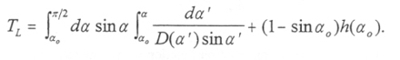
for q=2 [Kennel and Petschek, 1966; Kennel, 1969; Treumann and Baumjohann, 1997]. The lifetime T_L of the quasi-trapped particles is the total number of quasi-trapped particles in α_o<α<π/2 (Equation [2.36]) divided by the diffusion flux into the loss cone <S>. When the sources are assumed to inject particles at α=π/2, the lifetime has the form

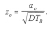
At this point it is convenient to make a distinction between the two limits on pitch angle diffusion. The diffusion strength is parameterized by the quantity

The limit where z₀ >> 1 corresponds to weak diffusion. In weak diffusion, there are many more particles at the edge of the loss cone (α≈α_o) than at the center (α=0), and many more near flat pitches than near the loss cone. In this limit, loss can match injection and the loss cone distribution increases exponentially from α=0 to α=α_o according to the asymptotic representation of the Bessel function. Therefore h is small outside the loss cone and Equation [2.41] becomes in the weak diffusion limit

If q>2 then T_L --> infinity as α decreases so particles can never diffuse to zero pitch before they are lost, and the pitch angle distribution has a hole at α=0. In the limit where z₀<<1, particles can be scattered across the loss cone in times comparable to or less than T_B, which is known as the strong diffusion limit. In this case D₀T_B >> 1 and the Bessel functions can be expanded in the small amplitude limit yielding

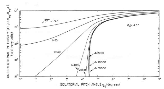
for all q. Equation [2.44] does not depend on the pitch angle within the loss cone. The pitch angle distribution is then flat between α<=α_o for strong pitch angle diffusion, and the loss cone is filled with particles. Figure 2.10 shows the solution to Equation [2.36] for various values of D₀T_B and a loss cone edge of a_o= 4.5°. Note that for large values of D₀T_B the loss cone is filled in, and for small values of D₀T_B the loss cone falls off exponentially and is shallow [Theordoridis and Paolini, 1967].

Figure 2.10 Numerical solution of Equation [2.36] done by Theodoridis and Paolini [1967]. Large DT_B corresponds to near strong diffusion, and small DT_B corresponds to weak diffusion.

Next: 2.5 Electric Fields

Return to dissertation table of contents page.

Return to main Galileo Table of Contents Page.
Return to Fundamental Technologies Home Page.

QUICK FACTS

RELATED LINKS