


Investigation of the Magnetosphere of Ganymede with Galileo's Energetic Particle Detector
Ph.D. dissertation by Shawn M. Stone, University of Kansas,
1999.
Copyright 1999 by Shawn M. Stone. Used with permission.
5.3 Implementation of Pitch Angle Scattering
In Chapter 2 the concept of pitch angle diffusion was discussed. For reasons that will become evident in Chapters 6 and 7, it is necessary to add pitch angle scattering to the simulation. Due to the small amount of time that the charged particles are in the Ganymede region [Williams et al., 1997], the pitch angle scattering mechanism is believed to be along the Jupiter field line. The exact mechanism for the scattering is not important; the fact that it has a stochastic effect on the particle pitch angles is all that is relevant. It should be emphasized here that the simulation does not seek to evaluate the cause of the mechanism, it only intends to emulate the effect of the mechanism on the particle pitch angle.
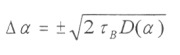
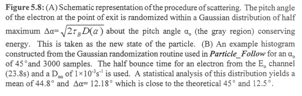
Pitch angle scattering is enforced in extended bounce mode. When the particle reaches the edge of S (as in position 1 in Figure 5.7a), its pitch angle is randomized within a Gaussian distribution centered around the pitch angle ao (the pitch angle at the edge of S), shown in Figure 5.8a. The width of this distribution at half maximum is from Equation [2.1] where it is assumed that the scattering is equally likely to increase as well as decrease the pitch angle.
|
[5.8] |
The form of D(a) used in the simulation at this time is constant within the loss cone D(a)=Daa. When a particle is leaving the bounce sphere, its pitch angle is between 0° and 90°. Figure 5.8b shows a histogram from the Gaussian random generator used in Particle_Follow for an ao of 45°, tB=23.8 s, and Daa= 1 x 10⁻³ s-1 for 3000 consecutive random numbers. The distribution is indeed Gaussian with a half width of 12.18° as predicted by Equation [5.8].
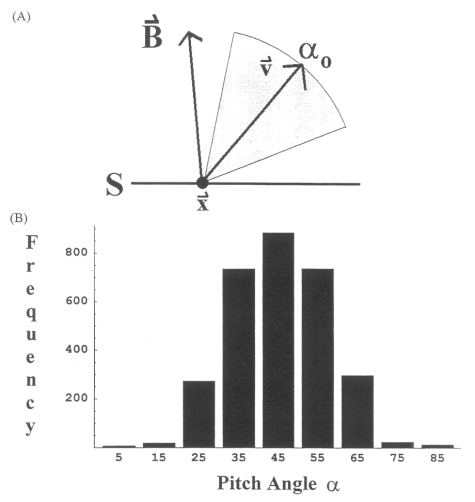
There are two limiting cases to consider: what happens when ao is near 0°, and when ao is near 90°. Figure 5.9a shows the situation of a particle whose ao is 15° where tB and Daa are the same as above. Pitch angles that are scattered below 0° are re-randomized. This gives a truncated Gaussian at 0°. Figure 5.9b shows the situation of a particle whose ao is 75°. Pitch angles that are scattered beyond 90° are also re-randomized, which gives a partial Gaussian distribution. This case happens infrequently, however, since particles with flat pitches do not make it out of the boundary S.
Figure 5.9 (A) Histogram example of a pitch angle ao=15°. The scattered pitch angles that fall below 0° are re-sampled back into the scattering bounds. Since this is a truncated Gaussian distribution the mean is 17° and Da~=10.5°. (B) Histogram example of a pitch angle ao=75°. The scattered pitch angles that fall beyond 90° are re-sampled back into the scattering bounds. Since this is a truncated Gaussian distribution the mean is 73° and Da~=10.5°.
5.4 Electric Fields
The two electric fields considered in the simulation are the corotational and parallel electric fields as discussed in Chapter 2. The implementation of each is rather simple. For the corotational electric field, given in Equation [2.47], the magnetic field B is the background Jovian field at the respective encounter at R, and W= 1.65 x 10⁻⁴ rad/s z is the rotational rate of Jupiter in GSII. The amount of the corotational electric field that permeates the magnetosphere of Ganymede can be varied in this simulation. An example of the corotational drift velocity is given in Appendix C. The parallel electric field is even simpler to define. The magnitude of E|| is specified by the user, and the direction is parallel to the magnetic field, pointing away from Ganymede, at the position of the particle and only operates within the boundary S.
5.5 Force Pitch and Phase Mode
Each of the magnetic field models considered in this work has regions in the magnetosphere of Ganymede where the model pitch and phase deviates from the measured by a significant amount. A significant amount means that an absorption feature can be totally missed if the local model pitch angle is a little too flat at the spacecraft. However, this is not a good test of the magnetic field geometry as a whole. In these instances, it is necessary to enforce the measured pitch and phase angles on the particle in the model field. This is done rather simply by two rotations of a unit vector aligned with the z axis of the magnetic field coordinate system. This vector is rotated by the pitch angle about the y axis, then by the phase angle about the z axis. This vector is then transformed into GSII by the rotations defined in Section 3.5.3. This is the new velocity vector of the particle.
Next: 5.6 Stepping Through the Encounter: Constructing the Simulated Count Rate
Return to dissertation table of contents page.
Return to main
Galileo Table of Contents Page.
Return to Fundamental
Technologies Home Page.
Updated 8/23/19, Cameron Crane
QUICK FACTS
Mission Duration: Galileo was planned to have a mission duration of around 8 years, but was kept in operation for 13 years, 11 months, and 3 days, until it was destroyed in a controlled impact with Jupiter on September 21, 2003.
Destination: Galileo's destination was Jupiter and its moons, which it orbitted for 7 years, 9 months, and 13 days.